Kelly Allocation with Bayesian Updating

Introduction

Some time ago, when I was living in Adelaide, I was approached by two men who wanted to figure out how to allocate bets made in a horse racing, specifically for exotic bets such as the trinella (picking the top three horses in any order) and quinella (picking the top four horses in any order) bets. They wanted me to figure out a way to compute the Kelly criterion (see below) as means to exponentially increase their pool of money over repeated bets. A huge complication is that it is a parimutuel betting system, so the odds for the horses updates even just right before the start of the race! How they found me was quite interesting as well: it turns out my lecture slides on gambling and information theory piqued their interest, having found it after a search on Google, which proves the power of putting stuff out there on the Internet.

Suffice to say I solved the problem, but am not at privy to disclose the solution as part of my consulting contract. In this post, however, I am going to discuss the Kelly criterion, and how to combine Bayesian statistics with it.

Single vs. Repeated Bets

Say you wanted to make a once-off bet with a friend involving flipping a coin. Given that you have a pool of money $M$, then, to maximize your winnings, the optimal policy is that you should bet the entire stake of $M$. For a fair coin, the expected reward would be $M/2$.

But what if you get to bet with your friend multiple times?

We can easily see that the strategy used in a once-off bet does not apply here. If we were to bet the full amount each round, the chance of survival long enough to compound the initial pool of money would be very slim, so our expected reward would tend towards 0 as the number of bets increase. We can see that, at the very least, the main name of the game for repeated bets is survival, while thriving.

What, then, is the the optimal strategy in this case?

Enter the Kelly Criterion

The Kelly criterion, developed by John L. Kelly Jr. at Bell Labs, is a strategy for the optimal sizing of bets in the repeated bets scenario in his seminal paper¹. Kelly himself was an interesting character: a chain smoking Texan who used to be a fighter pilot in the Navy during World War 2, he was also brilliant researcher. He developed the criterion as an alternative interpretation of information entropy, developed by his colleague, Claude Shannon. You can learn about its history from this fascinating book ².

Given an initial pool of wealth, the objective is to maximize the doubling rate of wealth as bets are being placed. The initial analysis on the case of horse racing in Kelly’s paper assumed that the bettor fully invested her portfolio over all options; variations later existed where the bettor can withhold a portion of wealth. What is interesting is that it can be mathematically proven that (almost surely) no other strategy would beat the Kelly criterion in terms of higher wealth in the long run.

The long short of it is that the Kelly criterion’s objective is to maximize the rate at which wealth doubles by allocating intelligently each time bets are being placed. Even if you know the odds are good, it’s not a good idea to go all in, since there is a chance of loss.

Let’s consider repeated bets on the coin toss scenario. In this case, the Kelly criterion is simply (example taken from Wikipedia)

$f^{*} = \frac{p(b + 1) - 1}{b}$

• $f^{*}$ is the fraction of the current wealth to bet (expressed in fraction),
• $b$ is the net odds received on the bet (e.g. betting $10, on win, rewards $14 (plus bet); then $b=0.4$), and
• $p$ is the probability of a win. If we let $q = 1 - p$, then interestingly, the Kelly criterion recommends that the bettor only bets ($f^*$ > 0) if the bettor has an edge, that is $b > q/p$ (note that $f^*$ can be negative if $b < q/p$ which means that the bettor should take the other side of the bet). It also says not to bet anything if $b = q/p$.

I’m not going to delve too much into the formula for this case in order to get to the good stuff below. You can find the derivation in standard textbooks like Thomas and Cover’s text³.

Now that we have built our intuition about the Kelly criterion, by contrasting the single bet case versus the repeated bets case, we can see a clear differences

• If the odds don’t favor you, don’t bet! This is equivalent to folding your cards in poker often, only sizing a large allocation for bets which favor you,
• For a single once-off bet, we maximize the average (or expectation) of your winnings, but for repeated bets, we maximize the geometric mean of your winnings.

These in concert helps us maximize the rate at which our money $M$ doubles (or doubling rate) each time.

This has been applied to various games, including horse racing, and even stock market investing. In the latter, it has been said that Warren Buffett himself is an Kelly bettor⁴ (although I would argue Charlie Munger is more of one than Buffett).

One Major Caveat

However, the major difficulty in applying the criterion is that it assumes that the true probabilities of events occurring is known to the bettor. In the coin toss example above, the bettor knows what the value of $p$ is, and she can size the bets accordingly.

In reality, these are often unknown and the probabilities have to be estimated by the bettor. Unfortunately, any estimate is by definition likely to be wrong. The criterion is sensitive to the estimated probabilities, and since the criterion maximizes the wealth doubling exponent, mistakes made in the estimated probabilities can easily ruin the bettor over time.

Note that in my consulting gig, my clients claim to have a system to estimate the probabilities of horses winning, so that made my job a lot simpler.

If you don’t such a system though, this is where Bayesian updating comes in. The goal is simple: we want to approximate the probabilities of events occurring based on all available information. We constantly update the probabilities in light of new information, then use this information to size our bets.

Example: Horse Racing!

For concreteness, let’s cast the problem to the specific problem of betting on horses at a race track. Let us assume that there are $K$ horses. In each round, we want to bet on a winning horse for that round, and once the round is over, the winner is one of the $K$ horses. Based on that information, we would want to update a set of probabilities $p_1, p_2, \cdots, p_K$, where $p_i$ is the probability that that horse $i$, over time to get closer and closer to the truth.

Check out the link here to run a simulation of how they all work together! Assuming you have Docker installed on your machine, just run the notebook via the provided script run.sh on your command line. The notebook is found in docker/Kelly Multiarm Portfolio Simulation.ipynb.

We assume that the horses perform independently. Based on this assumption, we can model the probabilities of the horses winning via a Dirichlet distribution. The rationale for this is as follows:

• each horse win can be treated as a categorical random variable, so if horse $k$ wins, then the realized random variable is $k$, then
• as a general case of the Bernoulli process, the conjugate prior of a categorical distribution is the Dirichlet distribution, hence, the choice of the Dirichlet distribution. This would be clearer in the Jupyter notebook.

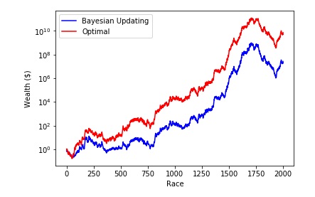
We will see that in simulations, over repeated bets due to errors in the estimated probabilities, the allocation is often imperfect and don’t approach the optimal allocation, that is, if the bettor knew the underlying horse win probabilities. We can see this in the following figure, where the initial wealth starts from $1 for both the optimal and Bayesian portfolios. The results are undeniable though: as the estimation gets better, the resulting allocations get much better too!

Final note

Of course, reality is far more complicated:

• we assume that the performance of horses are independent to each other: this may not be true in reality,
• the underlying true probabilities remain static throughout the simulation: again, the probabilities would be more dynamic in real life, coming from an unknown process more than anything else,
• the objective function assumes that there are no errors in the estimated probabilities: accounting for the uncertainty in the estimates could improve the allocation, and
• the odds remain static throughout the simulation: this is clearly not true in a parimutuel betting system, so it would be interesting to constantly update the probabilities in the face of changing odds.

One avenue I have not explored is to switch to a non-parametric model (a.k.a. neural networks) to estimate the probabilities. This is exciting because one could presumably use more contextual information about each horse, such as its jockey, past performance on different tracks etc. to derive the probability of winning instead of attaching a classic conjugate prior like what we’ve done above.

Another is that applying it to the stock market is more complicated as there is a wider range of stock prices which essentially can be modelled by a continuous distribution. That being said, it is conceivable that some combination of Monte Carlo simulations could help with the estimation.

One main insight I would like to end on is that the modelling of the probabilities and the sizing of the bets are essentially estimation and decision tasks respectively. This has strong ties to reinforcement learning and control systems, so combining knowledge from these areas would be an exciting area to explore!

References

¹ John L. Kelly, “A New Interpretation of Information Rate”, Bell System Technical Journal. 35 (4): pp. 917–926, 1956 link

² William Poundstone, “Fortune’s Formula: The Untold Story of the Scientific Betting System That Beat the Casinos and Wall Street”, 2006 link

³ Thomas M. Cover and Joy A. Thomas, “Elements of Information Theory”, 2nd ed., 2006 link

⁴ Mohnish Pabrai, “The Dhandho Investor: The Low-Risk Value Method to High Returns”, Wiley, 2007 link